CUDA Implementation of Parallel Bloom Tree

Introduction

Parallel Bloom Tree is a space-efficient representation for graphs using bloom filters to store graphs in a compact manner on GPU. MurmurHash3 has been used as the hash function in the bloom filter. The performance of the implementation is tested on the three algorithms namely Breadth First Search, Greedy Vertex Coloring and Tarjan’s Strongly Connected Components algorithm.

Code for the project can be found here.

Graph Operations

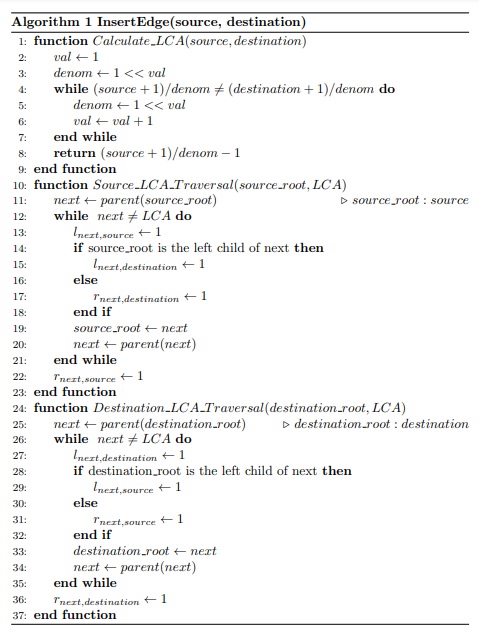
API: InsertEdge(p’, q’)

To insert an edge, the bits along the unique path between the two nodes, p’ and q’, must be set in accordance with the rules of Bloom Tree implementation. When inserting multiple edges in parallel, determining the unique paths between all the set of nodes first and then traversing the paths to set the values is not a feasible solution due to large memory requirement for the storage of the paths. A better method is to identify the Lowest Common Ancestor (LCA) [1] which is calculated using the function Calculate_LCA in the Algorithm 1 for all the set of nodes. Then, the function Source_LCA_Traversal is used to traverse upwards from the source nodes towards its LCA while simultaneously setting the appropriate bits as shown. Similarly, the function Destination_LCA_Traversal is used to traverse and set the appropriate bits in the bloom filter from the destination nodes to the LCA. The set of nodes are taken as source and destination and the algorithm is used to set the appropriate bits. In this case, the memory requirement is significantly reduced as only the corresponding LCA value needs to be stored for every edge to be inserted instead of the entire unique path.

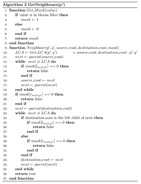
API: Neighbours of p’

This function can be used to identify the neighbours of a node. The node, p’, is checked if it is a neighbour to every other node parallelly. To check if the nodes are connected, first, their LCA is calculated [1]. The internal nodes are then traversed, one by one, from the nodes to their LCA while simultaneously checking if the appropriate bits are set. If the appropriate bit is set, then the traversal continues towards the LCA else it is stopped and it can be concluded that the nodes are not connected. If the LCA is encountered after traversal by both the nodes are completed, it is concluded that the nodes are connected and hence the other node, q’, is added as the neighbour of the node, p’. While checking if the appropriate bits are set in the bloom filter, the hash values are calculated multiple times for the same values. Hence, a mask is used as an optimization. The mask is a bool array which stores the values that have been set in the internal nodes. This bool array is calculated at the beginning of the function by checking the bloom filter as shown in Algorithm 2 using the function Get_Mask. It helps to avoid calculating the hash values and checking the bloom filters for every internal node in the tree traversal call as the value can be checked by seeing if it is set in the bool array instead.

API: IsEdge(p’, q’)

The function is used to check if an edge is present between two given nodes. The bits that have to be set for the edge to be present is first determined using the algorithm presented earlier. Then, these bits are checked if they are set parallelly using multiple threads. All the threads, before executing, make sure that any other thread, which has completed its execution, has not found a missing bit. If a missing bit is identified, the thread does not execute as there is no edge found.

Performance Evaluation

The defined functions were tested on a set of three algorithms, Breadth First Search (BFS), Greedy Vertex Coloring (VC), and Tarjan’s Strongly Connected Components (SCC), to assess their performance. The GPU device used was NVIDIA Tesla T4 on Google Colaboratory. Four graphs from the SNAP dataset [2] were chosen to run the algorithms.

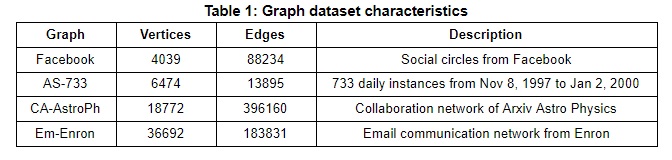
Test Data

The dataset to test the implementation was obtained from the Stanford Network Analysis Platform (SNAP) [2]. From the different types of dataset available, one graph each from the social network, communication network, collaboration network and autonomous systems graph was chosen. The characteristics of the chosen graphs are shown in Table 1.

Evaluation parameter

The Execution Time is the evaluation parameter considered. It is measured in ms. This is the time taken to run the algorithms assuming that the data is already present in the GPU. That is, the transfer time for data from CPU to GPU and vice versa are ignored.

Results and Discussion

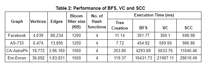
From the Table 2, we can observe that the time taken for tree creation is dependent on the number of edges and hence, the execution time for Graph CA-AstroPh is the largest. On the other hand, the time taken for the three algorithms is dependent on the number of vertices rather than the number of edges and accordingly the execution time increases as the number of vertices increases.

References

1. Wang, Xingbo. (2015). Properties of the Lowest Common Ancestor in a Complete Binary Tree. International Journal of Scientific and Innovative Mathematical Research. 3. 12-17.

2. Stanford Large Network Dataset Collection (SNAP) - http://snap.stanford.edu/data/